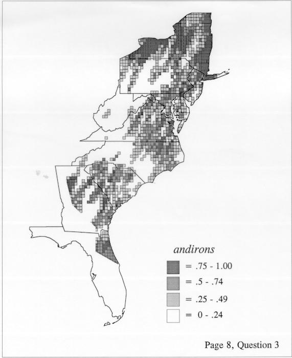
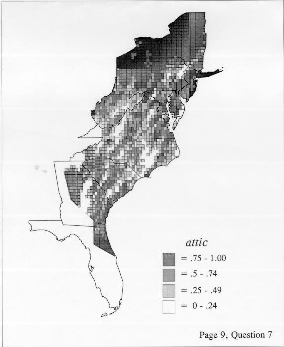
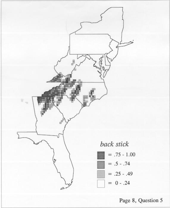
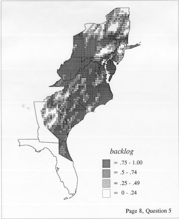
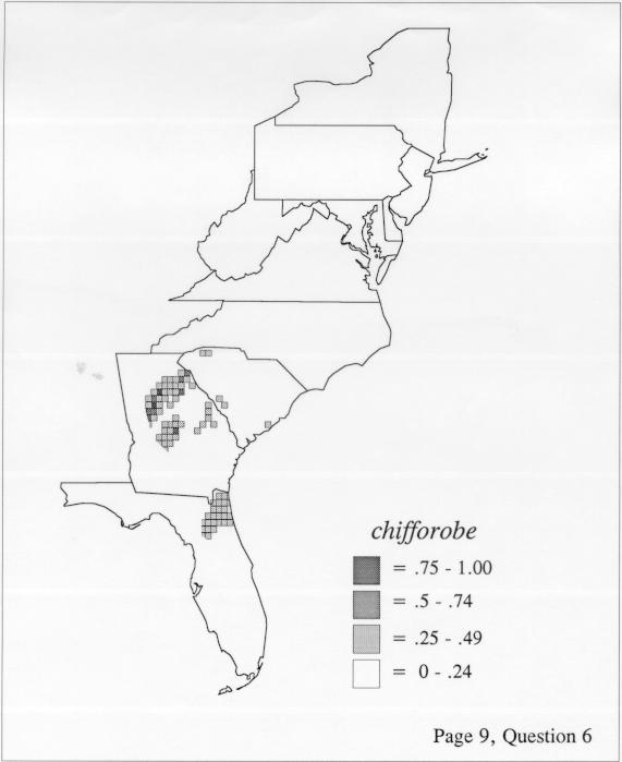
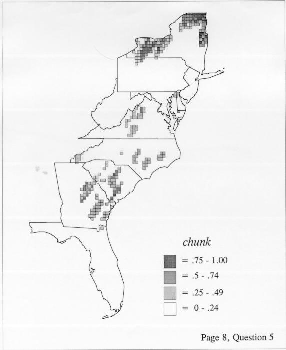
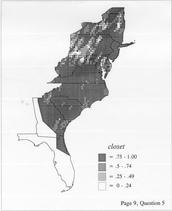
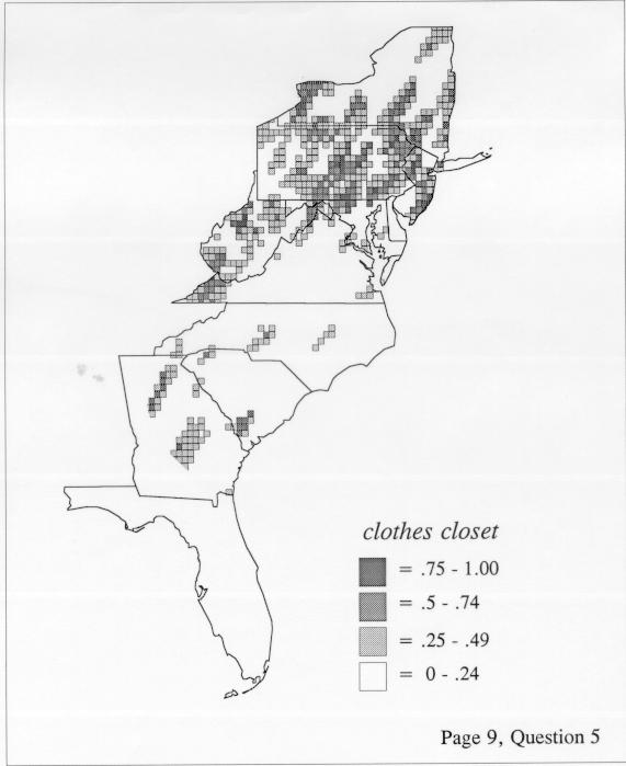
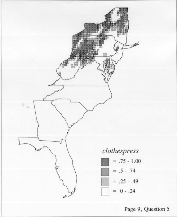
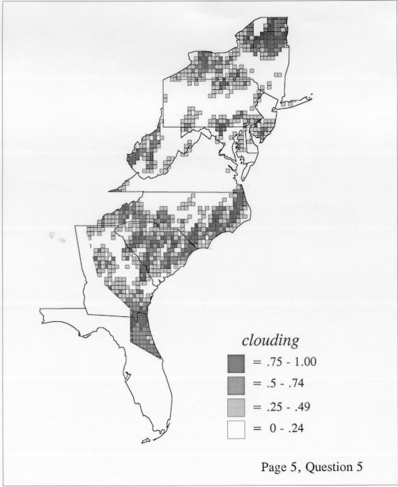
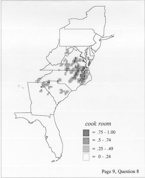
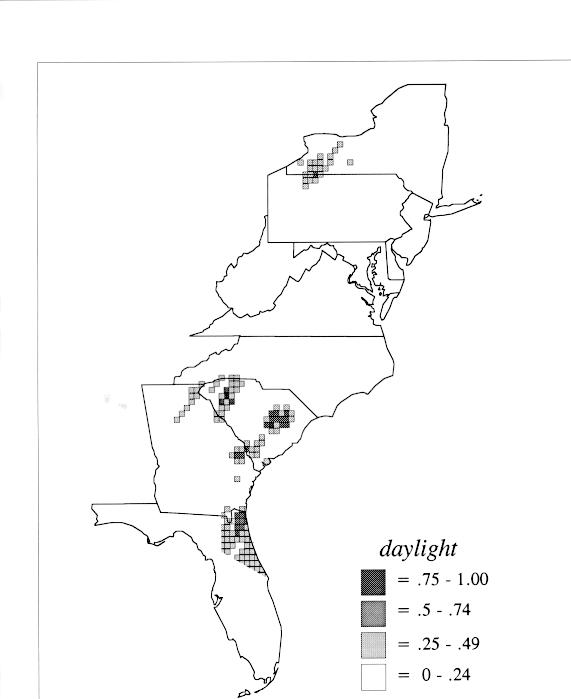
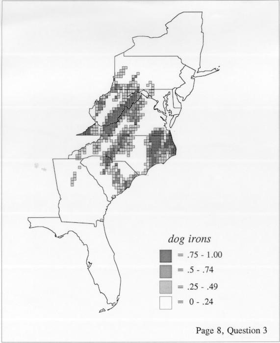
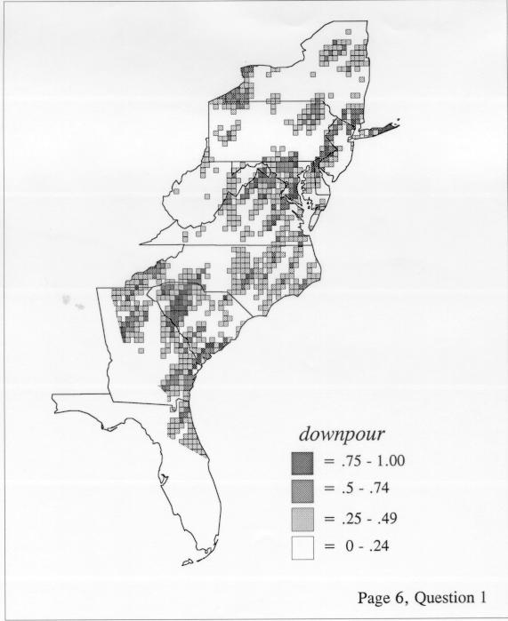
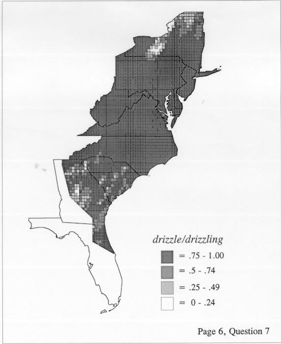
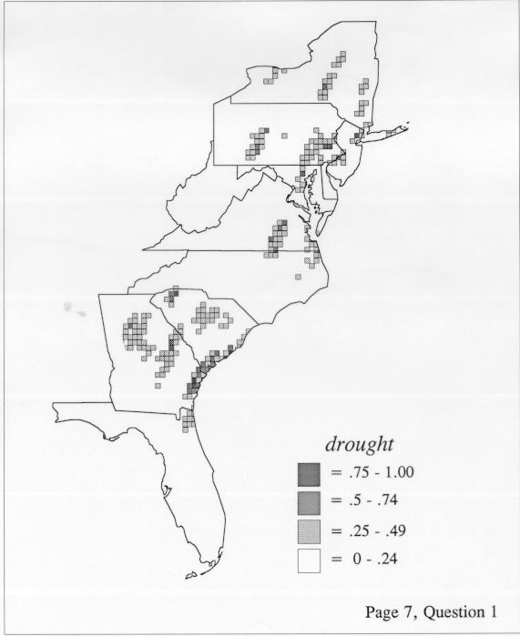
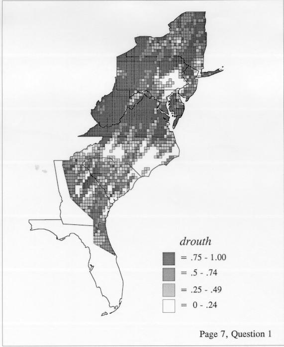
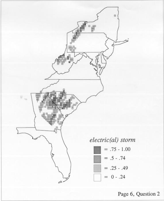
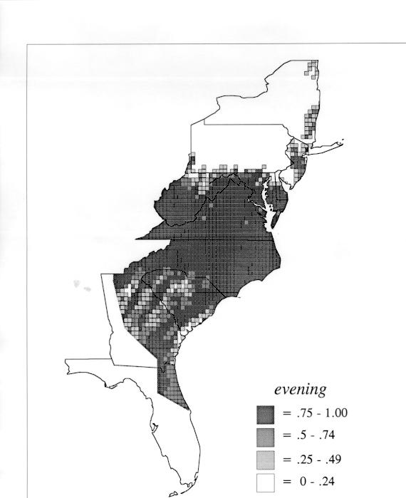
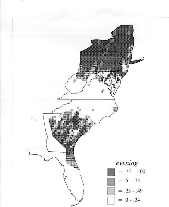
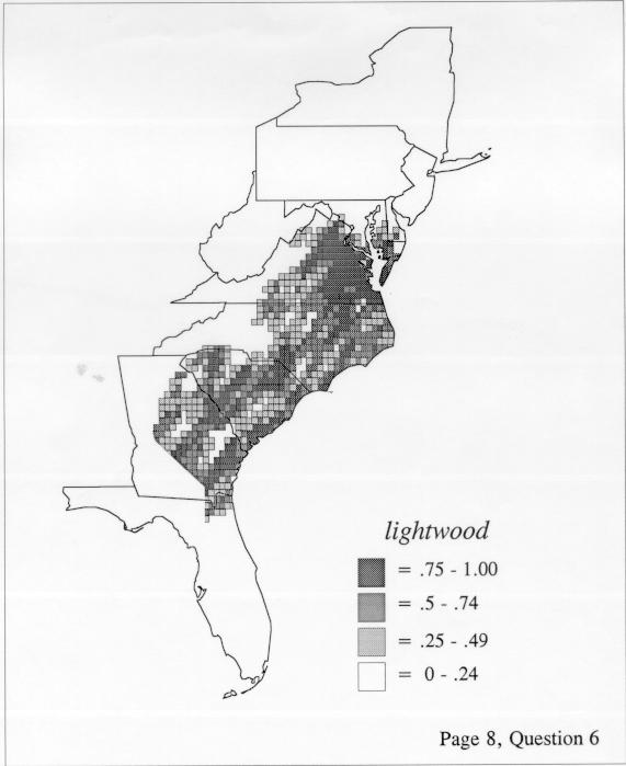
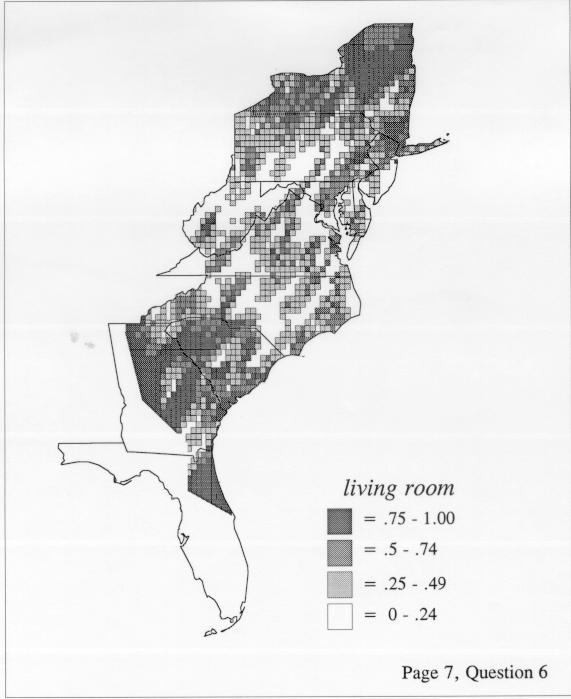
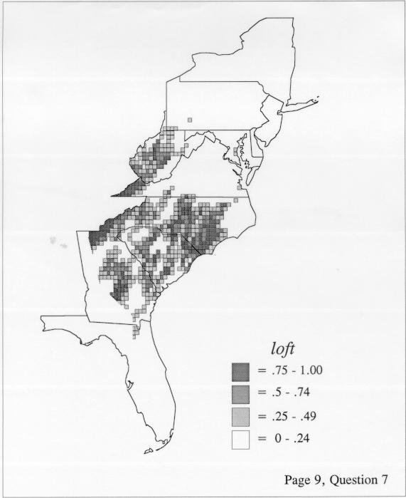
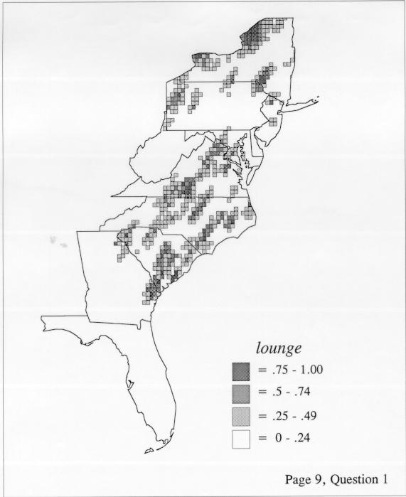
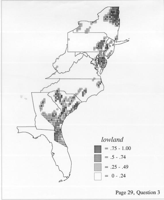
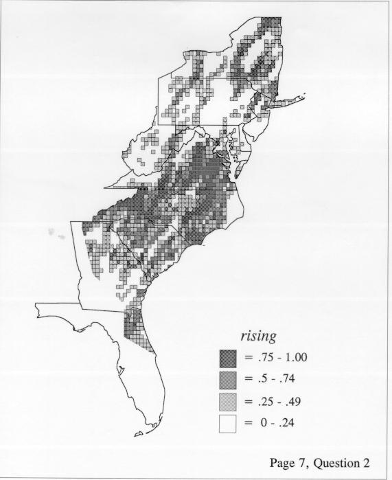
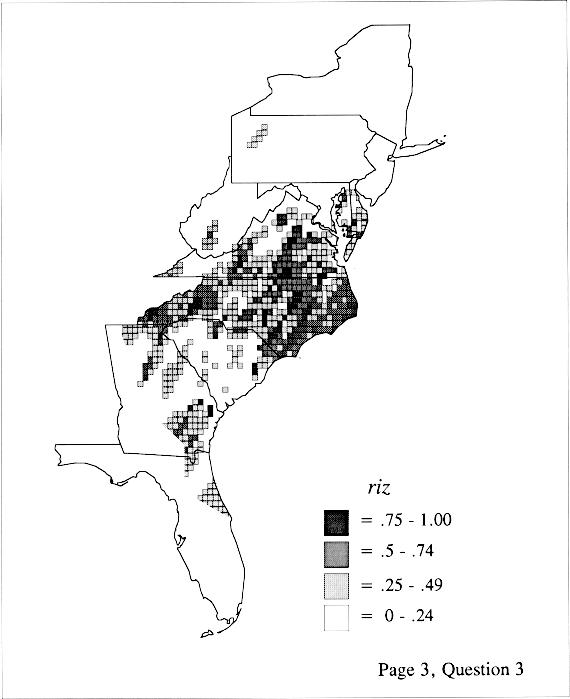
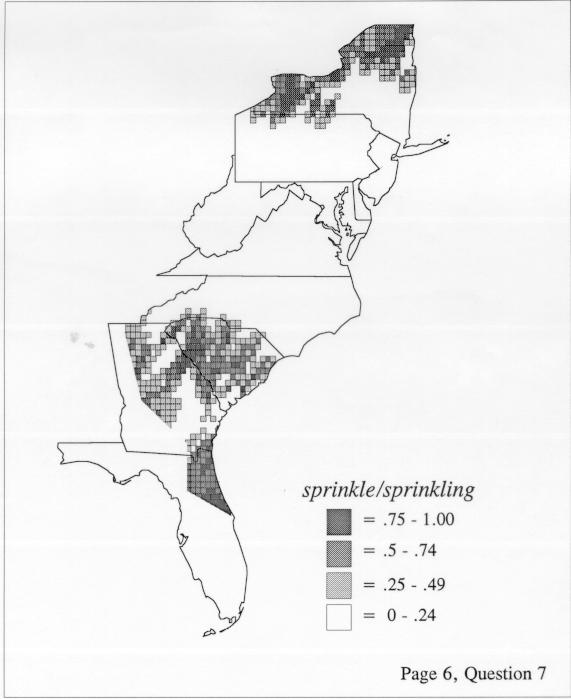
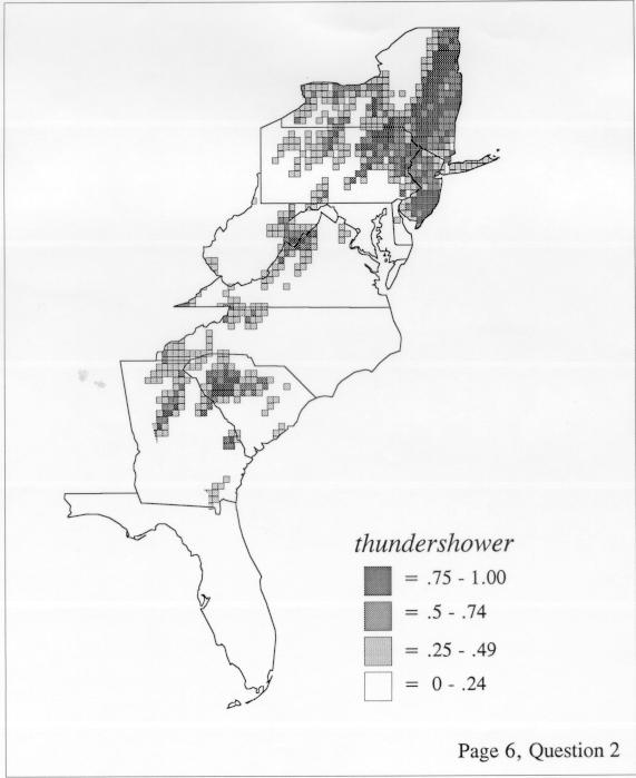
Density Estimation
Density estimation (DE) is a quantitative method. that can be used to show areal distributions for linguistic features. The procedure, a part of the Discriminant Analysis statistic in some statistical programs such as SAS, makes plots that show the density of occurrence of a feature, show the probability that a feature will occur in areas of a survey region, and predict comprehensively where a feature might be expected to occur in a survey region. The general assumptions for density estimation are that, for any single response to a particular elicitation cue, there will be a set of points (the locations where informants lived) where the response was elicited (call it “set A”) and another set at which it was not (call it “set B”). Reasonable information exists about which of the whole set of 1162 LAMSAS speakers were asked the question and which were not, and LAMSAS data files are so coded; set A and set B, for each test, are limited to those speakers who were asked the question (typically well over 90% of the total). We expect points from set A to be intermixed with points from set B: we are interested in finding out whether it is possible to define a best-fit geographical boundary within which there is a significantly higher proportion of points from set A than expected.
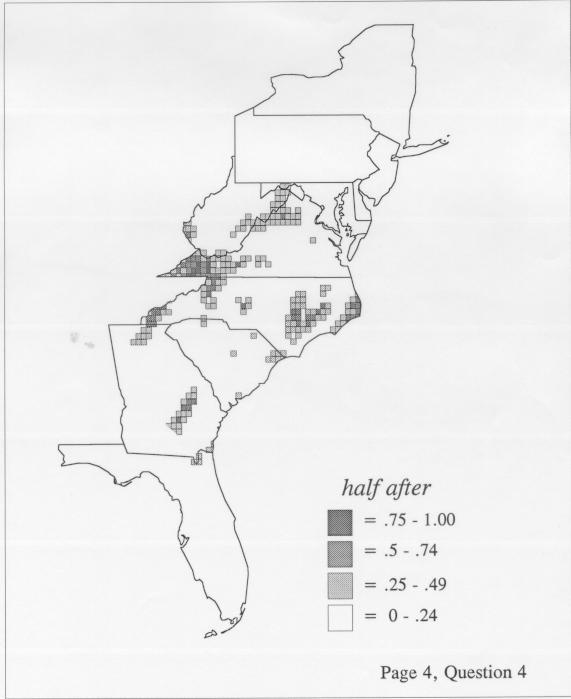
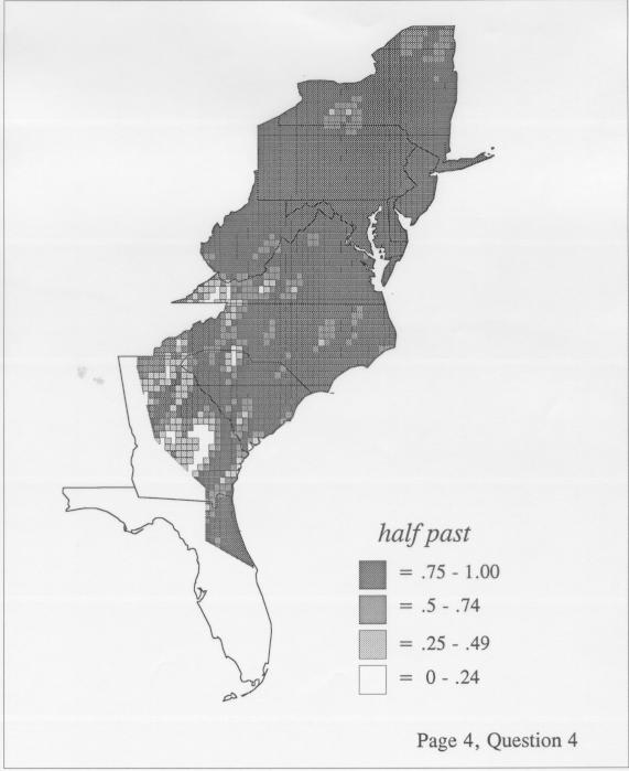
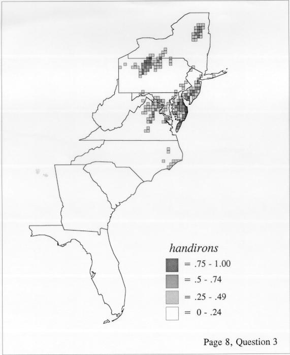
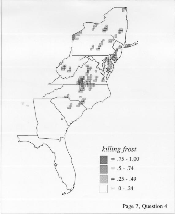
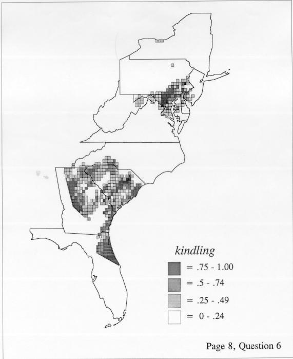
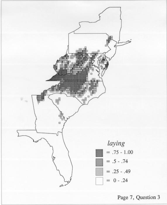
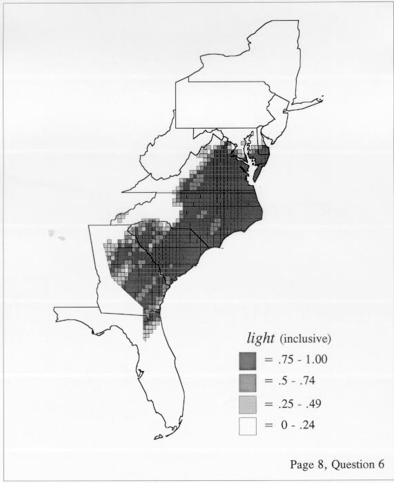
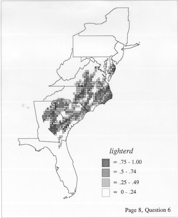
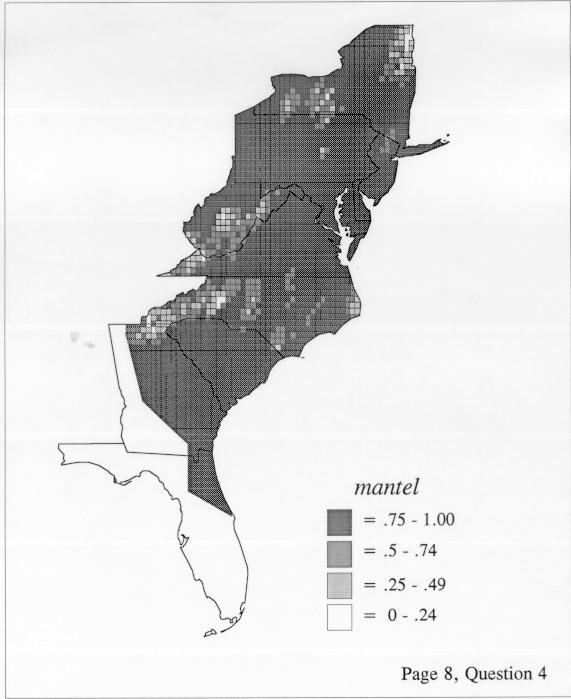
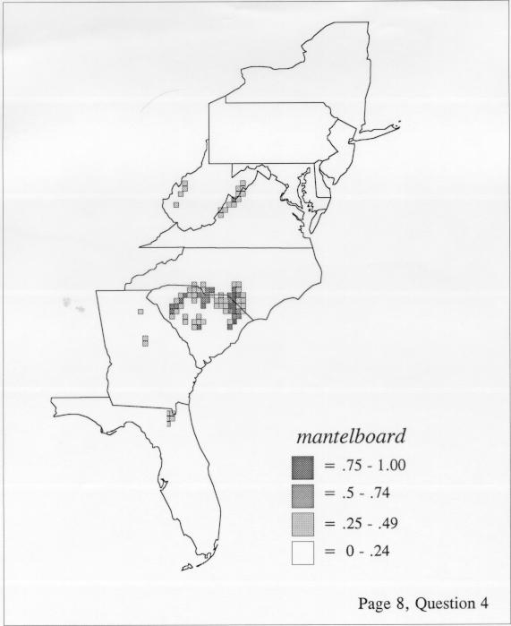
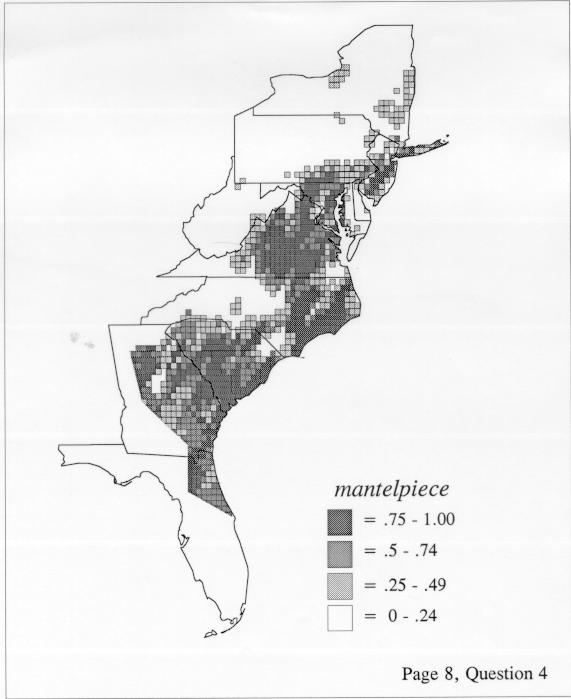
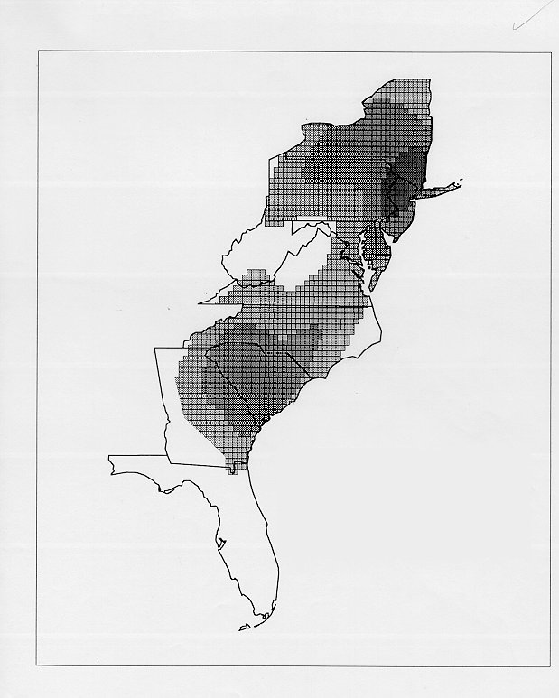
There are two basic nonparametric statistics for density estimation, the kernel method and the nearest-neighbor method. For the kernel method, the computer program uses a rather technical means to calculate the radius of a circle; this circle is then set around each of the speaker locations in turn, and the density of occurrence of the target linguistic feature within the circle is then calculated, again by rather technical means. The nearest-neighbor method begins differently but ends the same way. The investigator gets to choose how many nearest neighbors will be calculated for each location on a map. When the program calculates how all of the separate densities can yield a map of areal density overall, the map assumes that different areas are associated with each map location: under the kernel method the areas for each separate density are the same, but there are different numbers of speakers included for each area; under the nearest neighbor method, the same number of nearest neighbors for any given location may include a greater or lesser amount of territory.

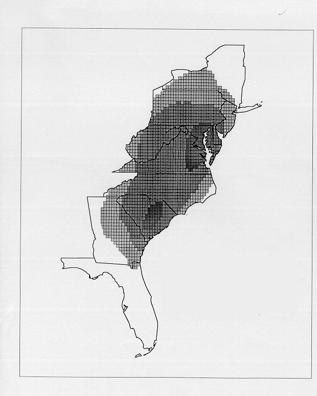
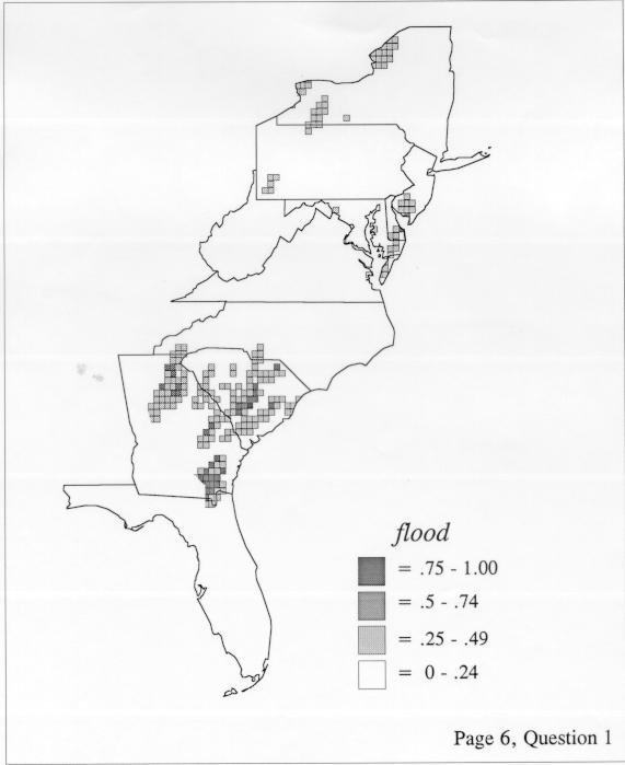
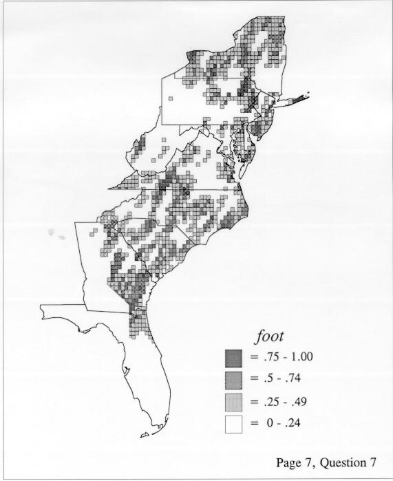
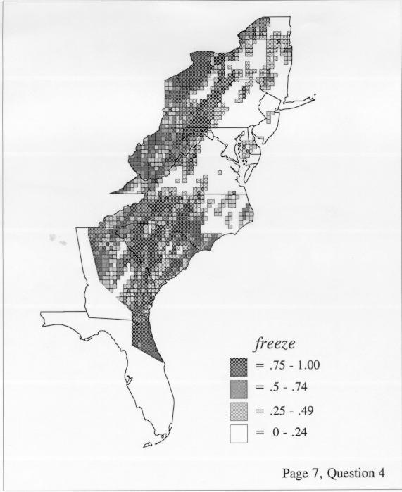
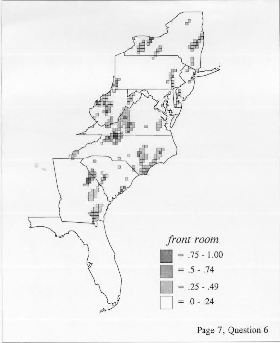
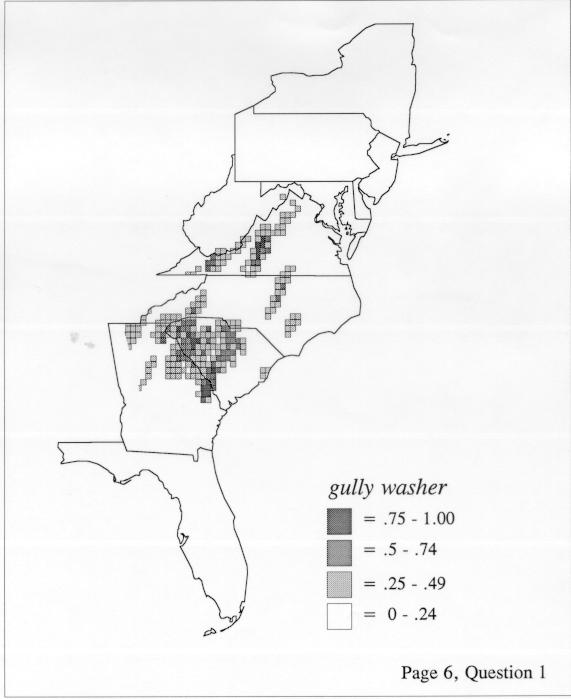
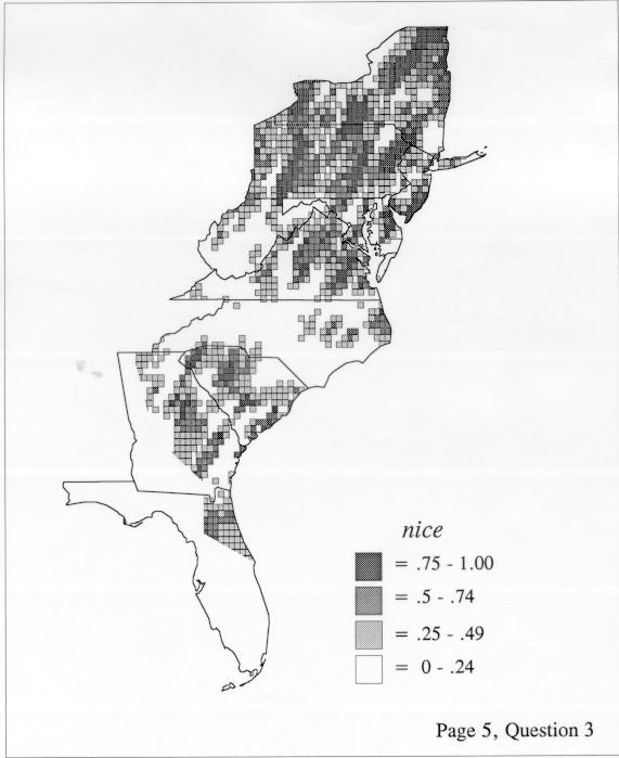
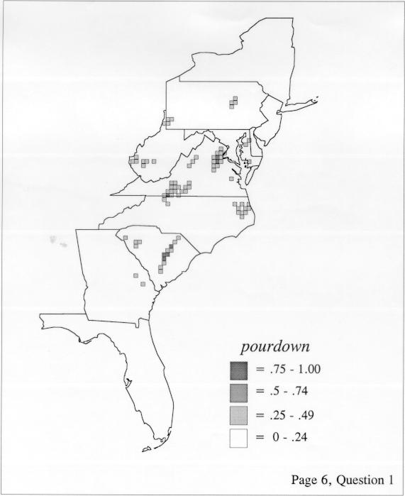
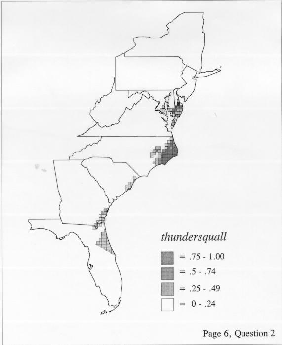
The differences in maps generated by the two methods can be shown from two items, bucket for the kernel method and cloudburst for nearest neighbors. The kernel method shows bucket in neat bullseye patterns centered in South Carolina and the Chesapeake Bay. The bullseye is characteristic of the kernel method, which has a “smoothing” coefficient that generates regular boundaries. On this kind of map one can draw the equivalent of an isogloss by distinguishing between predictions over 50% and predictions under 50%, which show two distinct areas.
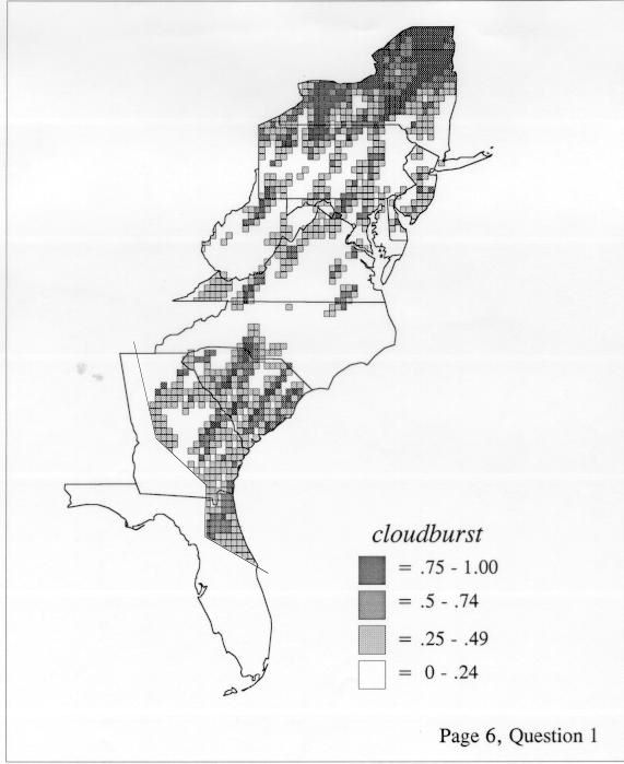
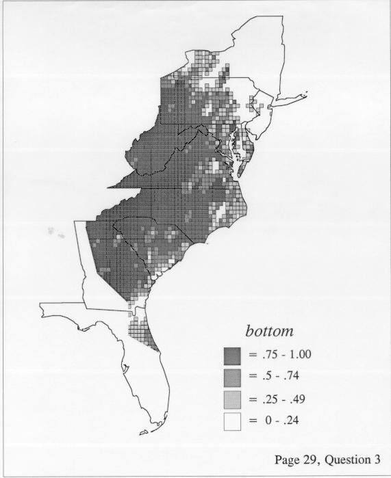
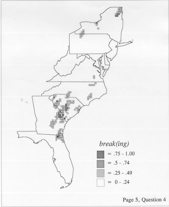
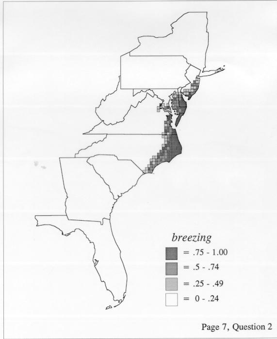
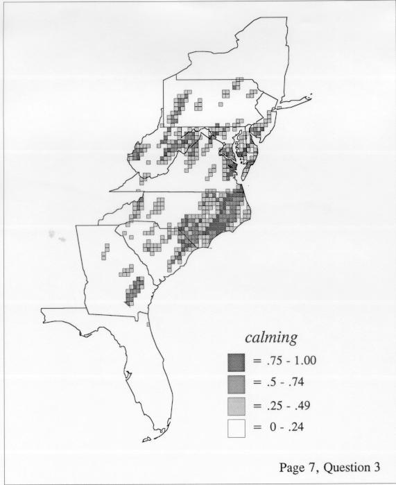
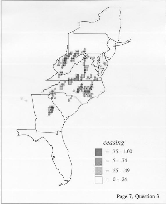
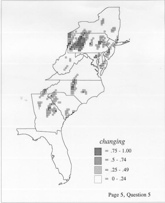
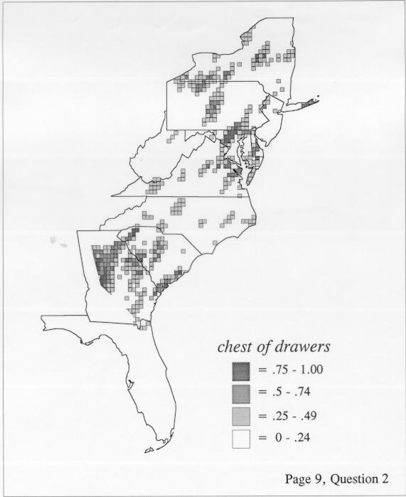
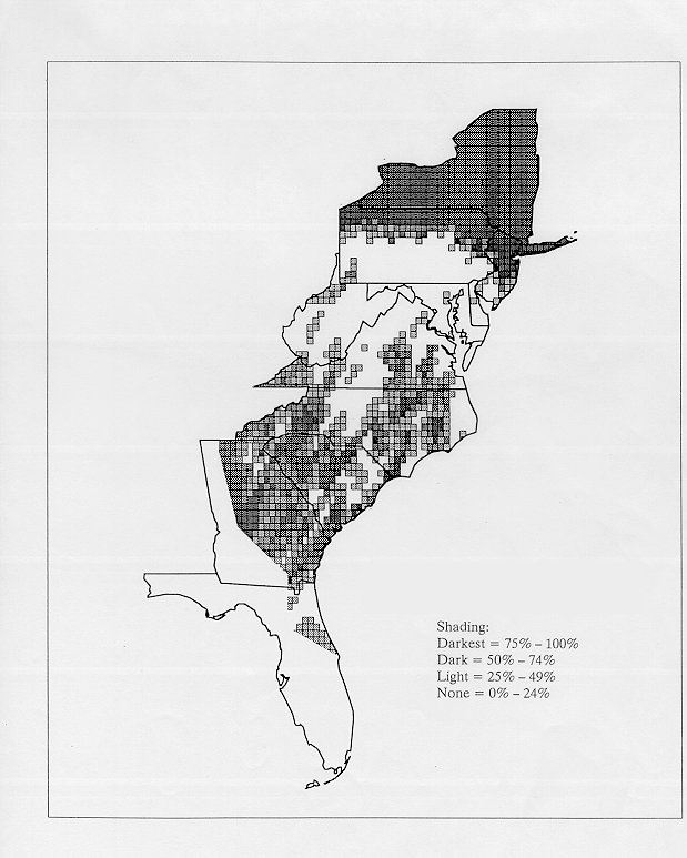
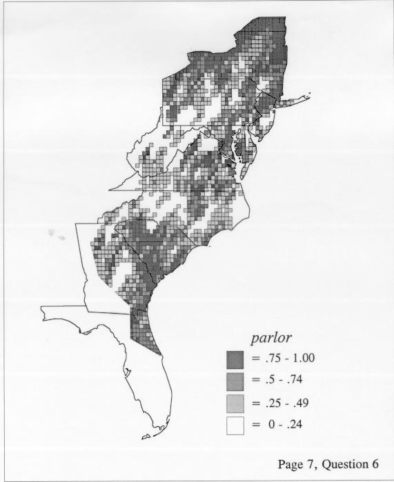
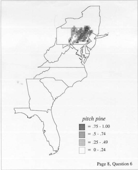
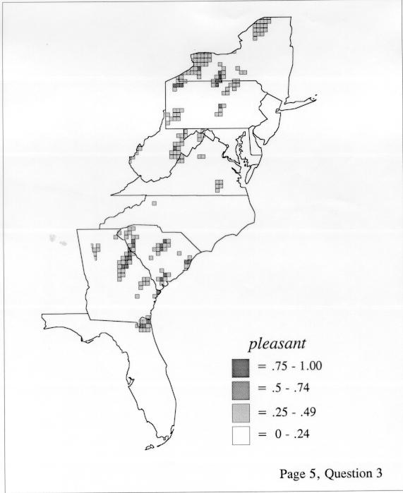
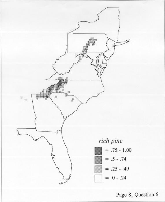
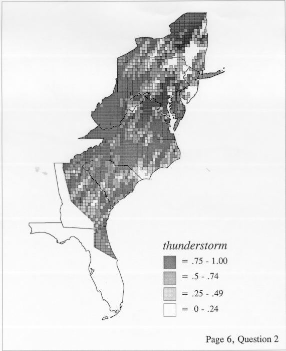
The smoothing coefficient of the kernel method tends to blur or hide small distributions. Better maps can be obtained with the nearest neighbor method. The cloudburst map shows many different areas of use of the word, here shown in four levels of shading where the darkest shading is the highest likelihood for occurrence of the word. While the kernel method shows homogenous regions because of its smoothing function, the nearest neighbor map shows that areas of use are actually scattered and lack coherence. That is, the consistent areas of the kernel map come from smoothing, and do not represent the actual distribution of the word as shown in the nearest neighbors map. This pattern of local clustering is also shown by the spatial autocorrelation statistic.
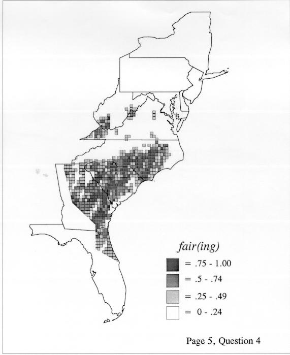
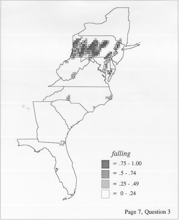
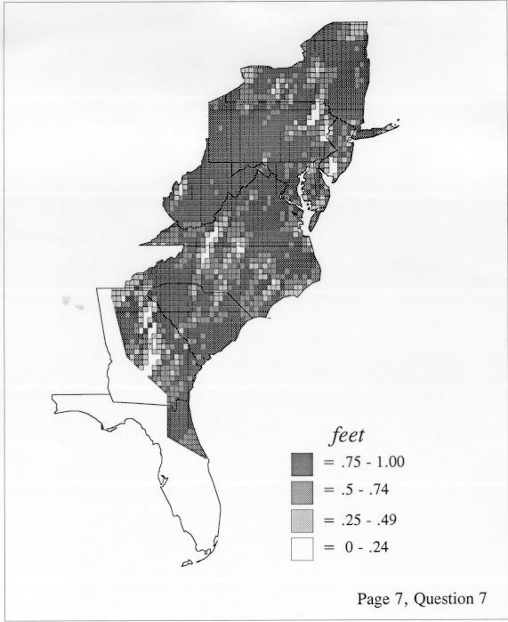
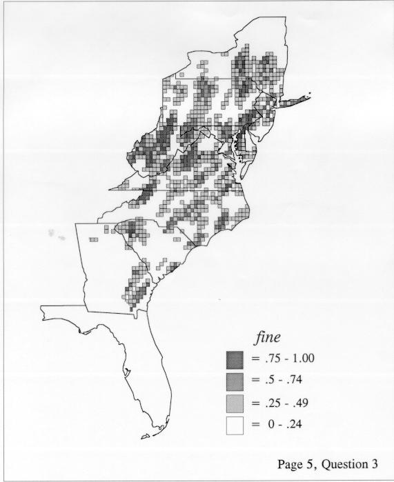
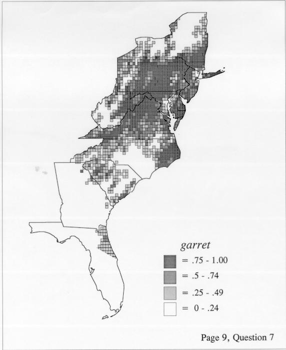
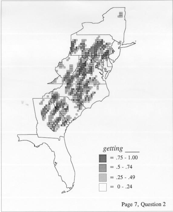
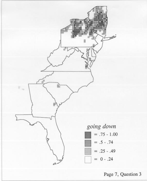
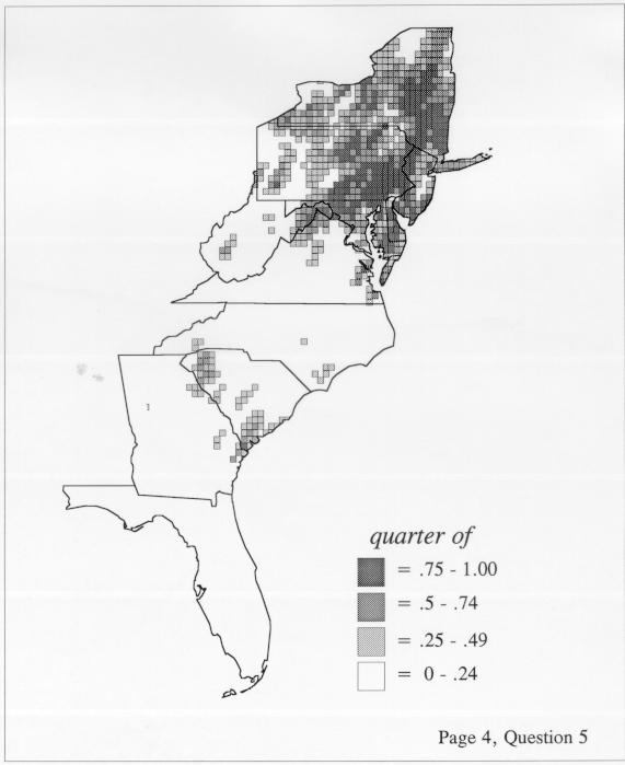
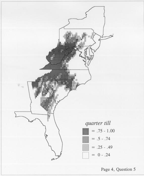
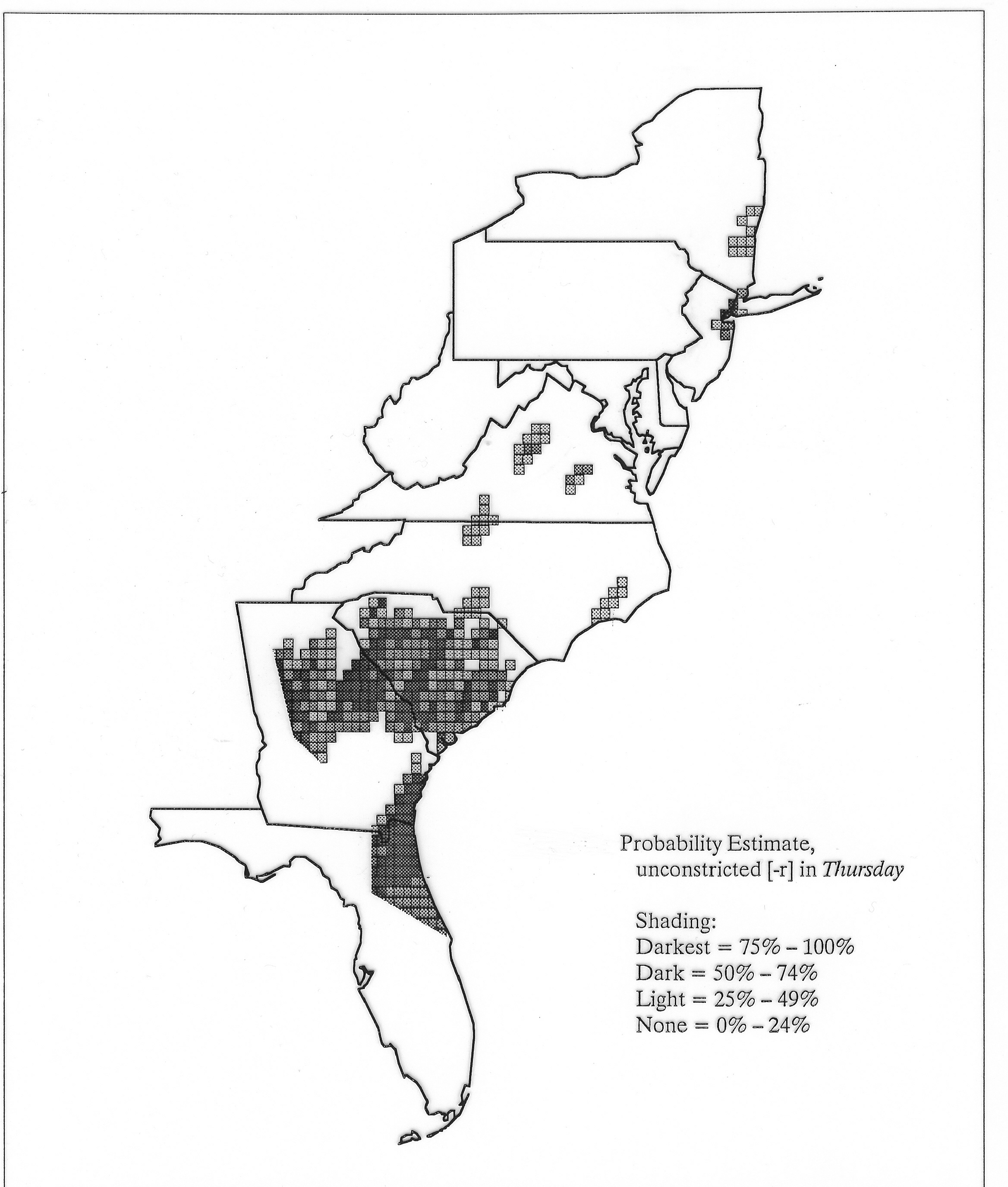
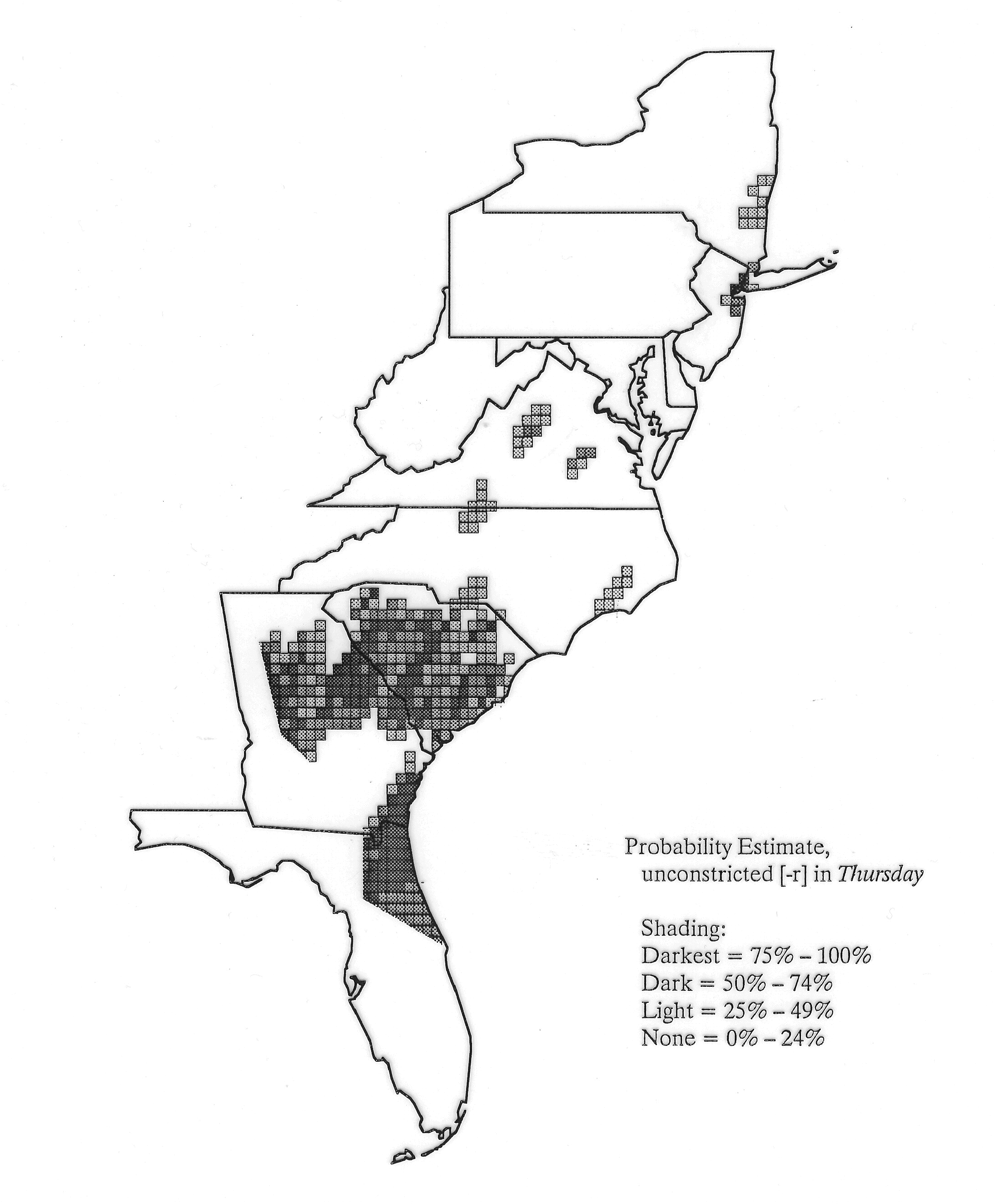
The set of DE maps in this collection were created by Deanna Light. Almost all of them use the nearest neighbor method.